Pandas: The Ultimate Library for Data Manipulation in Python

Unlock the full potential of your data with Pandas, Python’s powerhouse library for data manipulation and analysis. Whether you’re a seasoned data scientist or just diving into data analysis, Pandas offers the tools you need to transform raw data into actionable insights. Dive in to discover why Pandas is the go-to library for data enthusiasts worldwide.

Introduction

In the ever-evolving landscape of data science, Pandas stands out as a cornerstone library for data manipulation and analysis. Created by Wes McKinney in 2008, Pandas has revolutionized how analysts and scientists handle structured data, making complex operations straightforward and efficient. Let’s explore the facets that make Pandas indispensable in the data science toolkit.

What is Pandas?

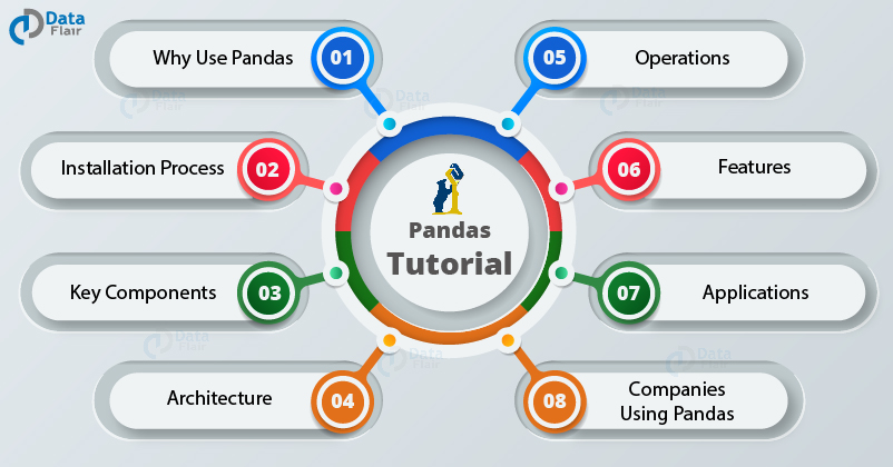
Pandas is an open-source Python library tailored for data manipulation and analysis. It provides two primary data structures:

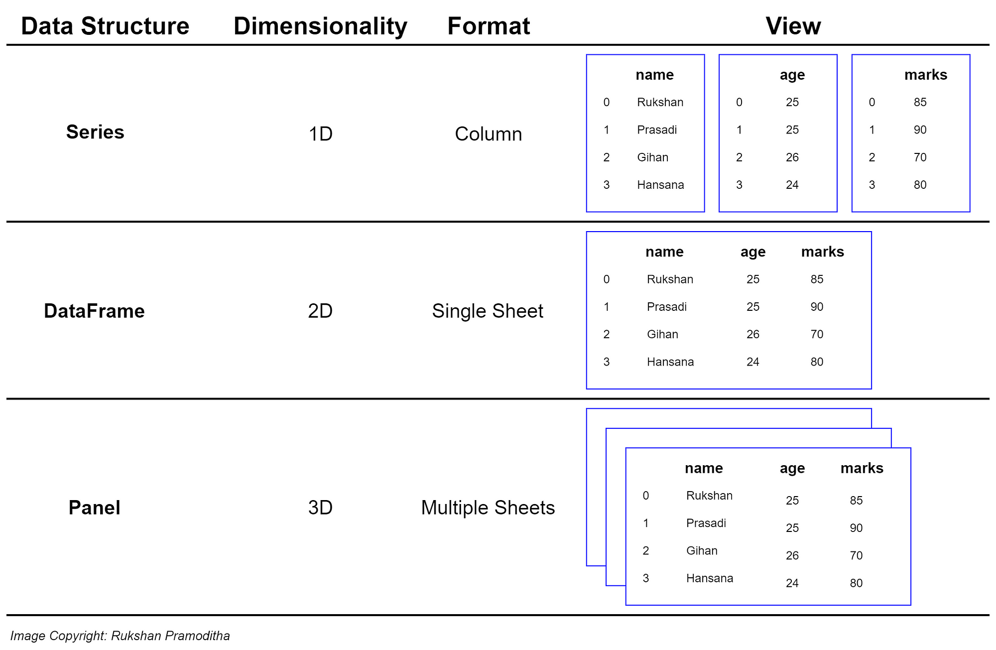
Series: A one-dimensional labeled array capable of holding any data type.
DataFrame: A two-dimensional labeled data structure with columns that can hold different data types, similar to a spreadsheet or SQL table.

These structures empower users to perform a wide array of operations efficiently, from simple data cleaning to complex transformations.

Feature	Series	DataFrame
Dimensionality	One-dimensional	Two-dimensional
Use Case	Single column data	Multiple columns, tabular data
Flexibility	Stores any data type per element	Stores different data types per column

Pandas excels in handling large datasets, providing functionalities for data cleaning, manipulation, and visualization. Its integration with other libraries like NumPy and Matplotlib amplifies its capabilities, making it a versatile tool for a variety of data science tasks.

Why Pandas is Essential for Data Science

Pandas is pivotal in the data science workflow for several reasons:

Data Cleaning: Simplifies the process of handling missing data, duplicates, and inconsistencies.
Data Transformation: Enables efficient reshaping, merging, and aggregation of datasets.
Exploratory Data Analysis (EDA): Facilitates quick insights through summary statistics and visualizations.
Integration: Seamlessly works with other libraries like NumPy, Matplotlib, and machine learning libraries such as Scikit-learn.

Key Benefits:

Efficiency: Optimized for performance with large datasets.
Flexibility: Handles various data formats including CSV, Excel, SQL databases, and more.
Ease of Use: Intuitive syntax that lowers the barrier to entry for data manipulation tasks.

Pandas not only enhances productivity by automating repetitive tasks but also reduces the potential for human error, ensuring that data analysis is both accurate and reliable. Its widespread adoption in industries like finance, healthcare, and marketing underscores its importance in transforming raw data into meaningful insights.

Key Features of Pandas

Pandas offers a rich set of features that cater to diverse data manipulation needs:

Data Structures: Series and DataFrame for flexible data handling.
Data Cleaning: Functions like ‘dropna()’, ‘fillna()’, and ‘isnull()’ to manage missing data.
Data Transformation: Methods for merging, joining, concatenating, and reshaping data.
Grouping and Aggregation: Powerful ‘groupby’ operations for summarizing data.
Time Series Analysis: Built-in support for handling and analyzing time-indexed data.
Visualization: Integration with Matplotlib for generating plots directly from DataFrames.
Performance Optimization: Techniques for handling large-scale data efficiently.

Feature	Description
Data Structures	Series and DataFrame for versatile data manipulation
Data Cleaning	Tools to handle missing, duplicate, and inconsistent data
Transformation	Methods to reshape, merge, and concatenate datasets
Grouping	Advanced grouping and aggregation functions
Time Series	Specialized tools for time-based data analysis
Visualization	Built-in plotting functions and integration with Matplotlib
Optimization	Efficient memory usage and performance tuning for large datasets

These features collectively make Pandas a robust tool for data scientists, enabling them to perform comprehensive analyses with ease and precision.

Getting Started with Pandas

Embarking on your Pandas journey begins with setting up the library in your Python environment. Whether you’re using pip or Anaconda, the installation process is straightforward, ensuring you can start manipulating data in no time.

How to Install Pandas in Python

Installing Pandas is simple and can be done using either pip or Anaconda. Here’s a step-by-step guide for both methods:

1. Installing with pip:

Prerequisite: Ensure Python is installed. Download from python.org if necessary.
Installation Command: bash pip install pandas
Advantages:
- Quick and easy installation.
- Access to the latest version via PyPI.

2. Installing with Anaconda:

Recommendation: Ideal for beginners due to its package management and deployment simplicity.
Download: Get Anaconda from anaconda.com.
Installation Steps:
- Open Anaconda Prompt.
- Create a new environment: bash conda create -n myenv python pandas
- Activate the environment: bash conda activate myenv
Benefits:
- Handles dependencies automatically.
- Provides a robust environment for data science projects.

Comparison Table:

Installation Method	Pros	Cons
pip	Lightweight, latest versions available	Manual dependency management
Anaconda	Simplified package management	Larger installation size

After installation, verify by running: python import pandas as pd print(pd.version)

This confirms that Pandas is correctly installed and ready for use in your projects.

How to Import and Set Up Pandas in Your Project

Once installed, importing Pandas into your Python project is straightforward. Here’s how to get started:

1. Importing Pandas: python import pandas as pd

Alias ‘pd’ is standard and widely recognized in the data science community.

2. Creating Data Structures:

Series Example: python data = [1, 2, 3, 4, 5] series = pd.Series(data)
DataFrame Example: python data = { ‘Name’: [‘Alice’, ‘Bob’, ‘Charlie’], ‘Age’: [25, 30, 35] } df = pd.DataFrame(data)

3. Importing Data from External Sources:

CSV Files: python df = pd.read_csv(‘data.csv’)
Excel Files: python df = pd.read_excel(‘data.xlsx’)

4. Verifying Data: python print(df.head())

Displays the first few rows of the DataFrame for a quick overview.

Setting up Pandas correctly ensures that you can efficiently manage and analyze your data, laying the foundation for deeper insights and more sophisticated analyses.

Understanding Pandas Data Structures

Pandas introduces two fundamental data structures: Series and DataFrame. Understanding these is crucial for effective data manipulation.

Series – One-Dimensional Data

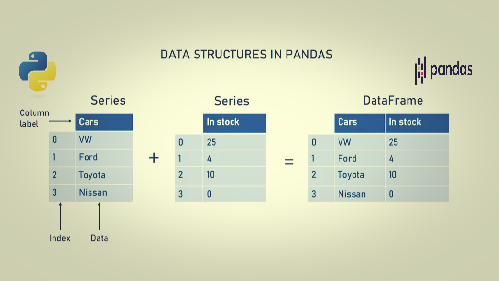
A Series is akin to a single column in a table. It holds data in a one-dimensional array, with an associated array of data labels, known as its index.

Key Characteristics:

Data Types: Can hold any data type (integers, strings, floats, Python objects).
Indexing: Each element is accessible via its index label.
Operations: Supports vectorized operations, making computations efficient.

Example: python import pandas as pd

Creating a Series

data = [10, 20, 30, 40, 50] series = pd.Series(data, index=['a', 'b', 'c', 'd', 'e']) print(series)

Output:

a 10 b 20 c 30 d 40 e 50 dtype: int64

DataFrame – Two-Dimensional Data

A DataFrame is a two-dimensional, size-mutable, and potentially heterogeneous tabular data structure with labeled axes (rows and columns).

Key Features:

Columns: Each column can hold different data types.
Indexing: Supports both row and column indexing.
Flexibility: Can be created from various data sources like lists, dictionaries, CSV files, databases, etc.

Example: python import pandas as pd

Creating a DataFrame

data = { 'Name': ['Alice', 'Bob', 'Charlie'], 'Age': [25, 30, 35], 'City': ['New York', 'Los Angeles', 'Chicago'] } df = pd.DataFrame(data) print(df)

Output:

”’
Name Age City
”’

0 Alice 25 New York 1 Bob 30 Los Angeles 2 Charlie 35 Chicago

Comparison Table:

Aspect	Series	DataFrame
Dimensionality	1D	2D
Usage	Single column data	Multiple columns, complex data
Flexibility	Homogeneous data types	Heterogeneous data types
Indexing	Single index	Row and column indexing

Mastering these data structures is essential as they form the backbone of data manipulation tasks in Pandas, allowing for efficient and effective data analysis.

Series – One-Dimensional Data

A Pandas Series is a one-dimensional array-like object that can hold a variety of data types, including integers, floats, and strings. Each element in a Series is associated with a unique index, making data retrieval straightforward and efficient.

Key Features:

Flexible Data Types: Can hold any data type, making it versatile for different datasets.
Indexed Data: Facilitates easy data access and manipulation through labels.
Vectorized Operations: Enables efficient computation without explicit loops.

Example Usage: python import pandas as pd

Creating a Series with custom index

data = [100, 200, 300, 400] index = ['A', 'B', 'C', 'D'] series = pd.Series(data, index=index) print(series)

Output:

A 100 B 200 C 300 D 400 dtype: int64

Series are particularly useful for representing individual columns of data and performing element-wise operations, which are integral to data analysis workflows.

DataFrame – Two-Dimensional Data

A DataFrame is a two-dimensional, size-mutable, and potentially heterogeneous tabular data structure with labeled axes (rows and columns). It is the most commonly used Pandas object for data analysis.

Key Features:

Multiple Columns: Each column can hold different types of data, akin to a table in a database or a spreadsheet.
Labeled Axes: Both rows and columns have labels, enabling precise data selection and manipulation.
Versatile Creation Methods: Can be created from lists, dictionaries, external files (CSV, Excel), and databases, offering flexibility in data ingestion.

Example Usage: python import pandas as pd

Creating a DataFrame from a dictionary

data = { ‘Product’: [‘Laptop’, ‘Tablet’, ‘Smartphone’], ‘Price’: [1200, 600, 800], ‘Stock’: [50, 150, 300] } df = pd.DataFrame(data) print(df)

Output:

”’
Product Price Stock
”’

0 Laptop 1200 50 1 Tablet 600 150 2 Smartphone 800 300

DataFrames are the cornerstone of data analysis in Pandas, enabling complex operations like grouping, merging, and pivoting with ease.

Data Handling and Processing with Pandas

Efficient data handling and processing are fundamental to deriving meaningful insights from data. Pandas provides a comprehensive suite of tools that streamline these processes, ensuring that data scientists can focus on analysis rather than data wrangling.

How to Load and Save Data Using Pandas

Loading and saving data are among the most common tasks in data analysis. Pandas simplifies these operations with intuitive functions tailored for various data formats.

Loading Data:

CSV Files: python df = pd.read_csv(‘data.csv’)
- Advantages:
  - Widely supported format.
  - Easy to read and write.
- Features:
  - Handles large datasets efficiently.
  - Supports various delimiters.
Excel Files: python df = pd.read_excel(‘data.xlsx’, sheet_name=’Sheet1′)
- Advantages:
  - Maintains data types and formatting.
  - Supports multiple sheets.
- Features:
  - Requires ‘openpyxl’ or ‘xlrd’ for reading Excel files.
JSON Files: python df = pd.read_json(‘data.json’)
- Advantages:
  - Suitable for nested data structures.
  - Easy to integrate with web APIs.
- Features:
  - Supports various JSON formats.
SQL Databases: python import sqlite3 conn = sqlite3.connect(‘database.db’) df = pd.read_sql(‘SELECT * FROM table_name’, conn)
- Advantages:
  - Direct integration with databases.
  - Efficient for large datasets.
- Features:
  - Supports various SQL engines via SQLAlchemy.

Saving Data:

CSV Files: python df.to_csv(‘output.csv’, index=False)
- Advantages:
  - Simple and universally accepted.
- Features:
  - Options for compression and custom delimiters.
Excel Files: python df.to_excel(‘output.xlsx’, sheet_name=’Sheet1′, index=False)
- Advantages:
  - Preserves data types and formatting.
- Features:
  - Supports multiple sheets and styling.
JSON Files: python df.to_json(‘output.json’, orient=’records’, lines=True)
- Advantages:
  - Ideal for web applications and APIs.
- Features:
  - Supports various JSON orientations.
SQL Databases: python df.to_sql(‘table_name’, conn, if_exists=’replace’, index=False)
- Advantages:
  - Directly writes to databases.
- Features:
  - Options for handling existing tables.

Comparison Table:

Format	Loading Function	Saving Function	Best For
CSV	‘read\_csv()’	‘to\_csv()’	Simple, flat data structures
Excel	‘read\_excel()’	‘to\_excel()’	Data with multiple sheets
JSON	‘read\_json()’	‘to\_json()’	Nested or web-based data
SQL	‘read\_sql()’	‘to\_sql()’	Large-scale database operations

Mastering these functions enables seamless data exchange between Pandas and various data sources, enhancing your ability to manage and analyze data effectively.

Reading Data from CSV, Excel, JSON, and Databases

Pandas provides specialized functions to read data from various formats, each suited to different types of data storage and retrieval needs.

CSV Files: python df = pd.read_csv(‘sales_data.csv’)
- Parameters:
  - ‘sep’: Specify the delimiter (default is comma).
  - ‘header’: Row number to use as column names.
  - ‘dtype’: Data type for data or columns.
Excel Files: python df = pd.read_excel(‘financials.xlsx’, sheet_name=’Q1′)
- Parameters:
  - ‘sheet_name’: Name or index of the sheet to read.
  - ‘usecols’: Specify columns to parse.
  - ‘engine’: Excel engine to use (‘openpyxl’, ‘xlrd’).
JSON Files: python df = pd.read_json(‘api_response.json’)
- Parameters:
  - ‘orient’: Indicate expected file format (‘records’, ‘split’, ‘index’).
  - ‘lines’: Read in lines format.
SQL Databases: python df = pd.read_sql(‘SELECT * FROM users’, conn)
- Parameters:
  - ‘sql’: SQL query string.
  - ‘con’: Database connection object.
  - ‘index_col’: Column to set as index.

Example: Reading from a SQL Database python import pandas as pd import sqlite3

Establish connection

conn = sqlite3.connect(‘company.db’)

Read data

df = pd.read_sql(‘SELECT employee_id, name, salary FROM employees’, conn)

Close connection

conn.close()

print(df.head())

Output:

employee_id name salary 0 1 Alice 70000 1 2 Bob 80000 2 3 Charlie 75000

This flexibility allows Pandas to interact seamlessly with diverse data sources, making it an indispensable tool for data analysts and scientists.

Writing Data to Different Formats

Once data is processed and analyzed, saving the results in various formats is essential for reporting, sharing, or further processing.

CSV Files: python df.to_csv(‘processed_data.csv’, index=False)
- Parameters:
  - ‘path_or_buf’: File path or object.
  - ‘sep’: Delimiter to use.
  - ‘columns’: Subset of columns to write.
Excel Files: python df.to_excel(‘processed_data.xlsx’, sheet_name=’Processed’, index=False)
- Parameters:
  - ‘sheet_name’: Name of the sheet.
  - ‘engine’: Excel writer engine (‘openpyxl’).
JSON Files: python df.to_json(‘processed_data.json’, orient=’records’, lines=True)
- Parameters:
  - ‘orient’: Format of the JSON string.
  - ‘lines’: Write JSON objects per line.
SQL Databases: python df.to_sql(‘processed_employees’, conn, if_exists=’replace’, index=False)
- Parameters:
  - ‘name’: Table name.
  - ‘con’: Database connection.
  - ‘if_exists’: Behavior if table exists (‘fail’, ‘replace’, ‘append’).

Example: Writing to an Excel File python import pandas as pd

Sample DataFrame

data = { ‘Product’: [‘Book’, ‘Pen’, ‘Notebook’], ‘Price’: [12.99, 1.99, 4.99], ‘Stock’: [100, 500, 300] } df = pd.DataFrame(data)

Save to Excel

df.to_excel(‘inventory.xlsx’, sheet_name=’Inventory’, index=False)

Output: An Excel file named ‘inventory.xlsx’ with a sheet labeled “Inventory” containing the data.

Best Practices:

Choose the Right Format: Select a format based on the end-use (e.g., CSV for simplicity, Excel for complex formatting).
Manage Indexing: Decide whether to include the DataFrame index based on relevance.
Handle Large Data: For large datasets, consider chunking or compression options to optimize storage and performance.

Effectively saving data ensures that your analysis results are preserved accurately and are easily accessible for future reference or further analysis.

How to Handle Missing Data in Pandas

Handling missing data is a critical step in data preprocessing. Pandas offers robust tools to identify, clean, and manage missing values, ensuring the integrity of your analysis.

Identifying Missing Values:

‘isnull()’ Function: Detects missing values. python missing = df.isnull() print(missing)
‘sum()’ Method: Counts missing values per column. python missing_count = df.isnull().sum() print(missing_count)

Removing Missing Data:

‘dropna()’ Function: Removes rows or columns with missing values. python df_cleaned = df.dropna(axis=0, how=’any’) # Drop rows with any NaN
- Parameters:
  - ‘axis’: 0 for rows, 1 for columns.
  - ‘how’: ‘any’ to drop if any NaN, ‘all’ to drop only if all are NaN.

Imputing Missing Values:

‘fillna()’ Function: Replaces NaN with specified values. python df_filled = df.fillna(value={‘Age’: df[‘Age’].mean()})
- Parameters:
  - ‘value’: Scalar, dictionary, Series, or DataFrame.
  - ‘method’: Forward fill, backward fill, etc.

Advanced Techniques:

Interpolation: Estimate missing values using interpolation methods. python df_interpolated = df.interpolate(method=’linear’)
Conditional Filling: Fill based on conditions or other column values. python df[‘Age’] = df.apply(lambda row: row[‘Age’] if pd.notnull(row[‘Age’]) else row[‘Age’].median(), axis=1)

Example: Handling Missing Data python import pandas as pd import numpy as np

Sample DataFrame with missing values

data = { ‘Name’: [‘Alice’, ‘Bob’, ‘Charlie’, ‘David’], ‘Age’: [25, np.nan, 35, 40], ‘City’: [‘New York’, ‘Los Angeles’, np.nan, ‘Chicago’] } df = pd.DataFrame(data) print(“Original DataFrame:”) print(df)

Identifying missing values

print(” Missing Values:”) print(df.isnull().sum())

Dropping rows with any missing values

df_dropped = df.dropna() print(” DataFrame after dropping missing values:”) print(df_dropped)

Imputing missing values

df_filled = df.fillna({‘Age’: df[‘Age’].mean(), ‘City’: ‘Unknown’}) print(” DataFrame after imputing missing values:”) print(df_filled)

Output:

Original DataFrame: Name Age City 0 Alice 25.0 New York 1 Bob NaN Los Angeles 2 Charlie 35.0 NaN 3 David 40.0 Chicago

Missing Values: Name 0 Age 1 City 1 dtype: int64

DataFrame after dropping missing values: Name Age City 0 Alice 25.0 New York 3 David 40.0 Chicago

DataFrame after imputing missing values: Name Age City 0 Alice 25.000000 New York 1 Bob 33.333333 Los Angeles 2 Charlie 35.000000 Unknown 3 David 40.000000 Chicago

Best Practices:

Understand the Cause: Determine why data is missing to choose the appropriate handling method.
Avoid Data Leakage: When imputing, ensure that the method does not introduce bias.
Document Changes: Keep track of how missing data is handled for transparency and reproducibility.

Effectively managing missing data is crucial for maintaining the accuracy and reliability of your analysis, paving the way for more credible and actionable insights.

How to Filter, Sort, and Aggregate Data

Filtering, sorting, and aggregating data are fundamental operations in data analysis. Pandas provides intuitive methods to perform these tasks efficiently.

Filtering Data:

Boolean Indexing: Select rows based on conditions. python filtered_df = df[df[‘Age’] > 30]
Using ‘query()’: Simplifies complex filtering. python filtered_df = df.query(‘Age > 30 and City == “Chicago”‘)

Sorting Data:

Sort by Column: python sorted_df = df.sort_values(by=’Age’, ascending=False)
Multiple Columns: python sorted_df = df.sort_values(by=[‘City’, ‘Age’], ascending=[True, False])

Aggregating Data:

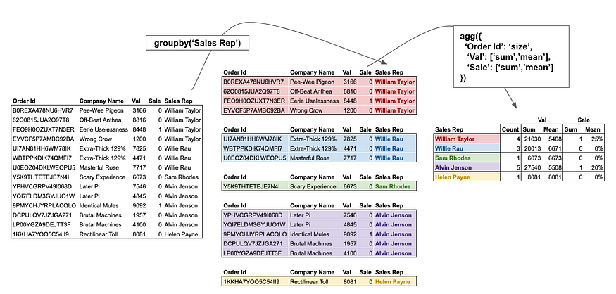
GroupBy Operations: python grouped = df.groupby(‘City’)[‘Age’].mean()
Aggregation Functions: python summary = df.groupby(‘City’).agg({ ‘Age’: [‘mean’, ‘min’, ‘max’], ‘Salary’: [‘sum’, ‘count’] })

Example: Filtering, Sorting, and Aggregating python import pandas as pd

Sample DataFrame

data = { ‘Department’: [‘Sales’, ‘Sales’, ‘HR’, ‘HR’, ‘IT’, ‘IT’], ‘Employee’: [‘Alice’, ‘Bob’, ‘Charlie’, ‘David’, ‘Eve’, ‘Frank’], ‘Age’: [25, 30, 35, 40, 28, 50], ‘Salary’: [50000, 60000, 70000, 80000, 55000, 90000] } df = pd.DataFrame(data)

Filtering: Employees older than 30

filtered_df = df[df[‘Age’] > 30] print(“Filtered DataFrame:”) print(filtered_df)

Sorting: By Salary descending

sorted_df = df.sort_values(by=’Salary’, ascending=False) print(” Sorted DataFrame by Salary:”) print(sorted_df)

Aggregating: Average salary per department

avg_salary = df.groupby(‘Department’)[‘Salary’].mean() print(” Average Salary per Department:”) print(avg_salary)

Output:

Filtered DataFrame: Department Employee Age Salary 2 HR Charlie 35 70000 3 HR David 40 80000 5 IT Frank 50 90000

Sorted DataFrame by Salary: Department Employee Age Salary 5 IT Frank 50 90000 3 HR David 40 80000 2 HR Charlie 35 70000 1 Sales Bob 30 60000 4 IT Eve 28 55000 0 Sales Alice 25 50000

Average Salary per Department: Department HR 75000.0 IT 72500.0 Sales 55000.0 Name: Salary, dtype: float64

Best Practices:

Chain Operations: Combine filtering, sorting, and aggregating for concise and readable code.
Use Descriptive Names: Clear variable names improve code readability.
Leverage GroupBy Flexibility: Utilize multiple aggregation functions to gain diverse insights.

Mastering these operations empowers you to distill large datasets into meaningful summaries and actionable insights, enhancing the decision-making process.

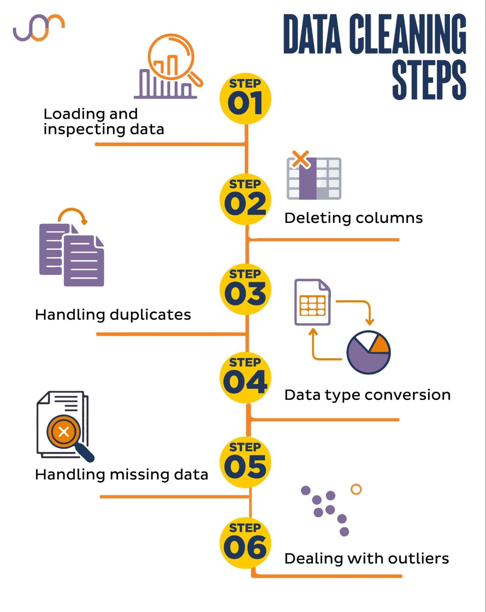
Data Transformation and Cleaning

Transforming and cleaning data are essential steps in preparing datasets for analysis. Pandas provides a suite of tools that simplify these processes, ensuring your data is accurate and ready for insightful analysis.

How to Modify Columns and Rows in a DataFrame

Modifying columns and rows is a common task in data preprocessing. Pandas offers various methods to adjust your DataFrame structure to better suit your analysis needs.

Modifying Columns:

Renaming Columns: python df.rename(columns={‘OldName’: ‘NewName’}, inplace=True)
Adding New Columns: python df[‘NewColumn’] = df[‘ExistingColumn’] * 2
Dropping Columns: python df.drop(‘UnnecessaryColumn’, axis=1, inplace=True)
Reordering Columns: python df = df[[‘NewColumn’, ‘ExistingColumn’, ‘AnotherColumn’]]

Modifying Rows:

Filtering Rows: python df_filtered = df[df[‘Age’] > 30]
Adding Rows: python new_row = {‘Name’: ‘Grace’, ‘Age’: 29, ‘City’: ‘Boston’} df = df.append(new_row, ignore_index=True)
Dropping Rows: python df.drop(index=0, inplace=True) # Drops the first row

Example: Modifying Columns and Rows python import pandas as pd

Sample DataFrame

data = { ‘Product’: [‘Laptop’, ‘Tablet’, ‘Smartphone’], ‘Price’: [1200, 600, 800], ‘Stock’: [50, 150, 300] } df = pd.DataFrame(data) print(“Original DataFrame:”) print(df)

Renaming a column

df.rename(columns={‘Stock’: ‘Inventory’}, inplace=True) print(” DataFrame after renaming ‘Stock’ to ‘Inventory’:”) print(df)

Adding a new column

df[‘Discounted_Price’] = df[‘Price’] * 0.9 print(” DataFrame after adding ‘Discounted_Price’:”) print(df)

Dropping a column

df.drop(‘Price’, axis=1, inplace=True) print(” DataFrame after dropping ‘Price’:”) print(df)

Adding a new row

new_product = {‘Product’: ‘Monitor’, ‘Inventory’: 100, ‘Discounted_Price’: 200} df = df.append(new_product, ignore_index=True) print(” DataFrame after adding a new product:”) print(df)

Output:

Original DataFrame: Product Price Stock 0 Laptop 1200 50 1 Tablet 600 150 2 Smartphone 800 300

DataFrame after renaming ‘Stock’ to ‘Inventory’: Product Price Inventory 0 Laptop 1200 50 1 Tablet 600 150 2 Smartphone 800 300

DataFrame after adding ‘Discounted_Price’: Product Price Inventory Discounted_Price 0 Laptop 1200 50 1080.0 1 Tablet 600 150 540.0 2 Smartphone 800 300 720.0

DataFrame after dropping ‘Price’: Product Inventory Discounted_Price 0 Laptop 50 1080.0 1 Tablet 150 540.0 2 Smartphone 300 720.0

DataFrame after adding a new product: Product Inventory Discounted_Price 0 Laptop 50 1080.0 1 Tablet 150 540.0 2 Smartphone 300 720.0 3 Monitor 100 200.0

Best Practices:

Maintain Consistent Naming: Use clear and consistent names for columns to enhance readability.
Avoid Duplicates: Ensure that adding rows or columns does not introduce duplicate entries unless intentional.
Handle Missing Data During Modification: Address missing values before or during the modification to maintain data integrity.

Effectively modifying your DataFrame structure allows for a more organized and meaningful representation of your data, facilitating deeper analysis and insights.

How to Merge, Join, and Concatenate DataFrames

Combining multiple DataFrames is a common requirement in data analysis, especially when dealing with related datasets. Pandas offers powerful functions to merge, join, and concatenate DataFrames seamlessly.

Merging DataFrames:

‘merge()’ Function: Combines DataFrames based on common columns or indices, similar to SQL joins. python merged_df = pd.merge(df1, df2, on=’key_column’, how=’inner’)
- Parameters:
  - ‘on’: Column to join on.
  - ‘how’: Type of join (”left”, ”right”, ”outer”, ”inner”).

Joining DataFrames:

‘join()’ Method: Simplifies joining on the index. python joined_df = df1.join(df2, on=’key_column’, how=’left’)
- Advantages:
  - Easier syntax when joining on indexes.
  - Supports multiple joins simultaneously.

Concatenating DataFrames:

‘concat()’ Function: Stacks DataFrames vertically or horizontally. python concatenated_df = pd.concat([df1, df2], axis=0) # Vertical stacking
- Parameters:
  - ‘axis’: 0 for rows, 1 for columns.
  - ‘ignore_index’: Reset index after concatenation.

Example: Merging, Joining, and Concatenating python import pandas as pd

Sample DataFrames

df1 = pd.DataFrame({ ‘EmployeeID’: [1, 2, 3], ‘Name’: [‘Alice’, ‘Bob’, ‘Charlie’] })

df2 = pd.DataFrame({ ‘EmployeeID’: [1, 2, 4], ‘Department’: [‘HR’, ‘Engineering’, ‘Marketing’] })

df3 = pd.DataFrame({ ‘EmployeeID’: [5, 6], ‘Name’: [‘Eve’, ‘Frank’] })

Merging DataFrames on ‘EmployeeID’

merged_df = pd.merge(df1, df2, on=’EmployeeID’, how=’inner’) print(“Merged DataFrame:”) print(merged_df)

Joining DataFrames using ‘EmployeeID’ as index

df1.set_index(‘EmployeeID’, inplace=True) df2.set_index(‘EmployeeID’, inplace=True) joined_df = df1.join(df2, how=’left’) print(” Joined DataFrame:”) print(joined_df)

Concatenating DataFrames vertically

concatenated_df = pd.concat([df1.reset_index(), df3], axis=0, ignore_index=True) print(” Concatenated DataFrame:”) print(concatenated_df)

Output:

Merged DataFrame: EmployeeID Name Department 0 1 Alice HR 1 2 Bob Engineering

Joined DataFrame: Name Department EmployeeID
1 Alice HR 2 Bob Engineering 3 Charlie NaN

Concatenated DataFrame: EmployeeID Name Department 0 1 Alice HR 1 2 Bob Engineering 2 3 Charlie NaN 3 5 Eve NaN 4 6 Frank NaN

Best Practices:

Ensure Key Consistency: The keys used for merging should have consistent data types and naming across DataFrames.
Choose the Right Join Type: Select the join type (‘left’, ‘right’, ‘inner’, ‘outer’) based on the desired outcome.
Handle Duplicates: Be cautious of duplicate keys that might result in unexpected row expansions.

Mastering these functions allows you to integrate diverse datasets seamlessly, enhancing the depth and breadth of your data analysis.

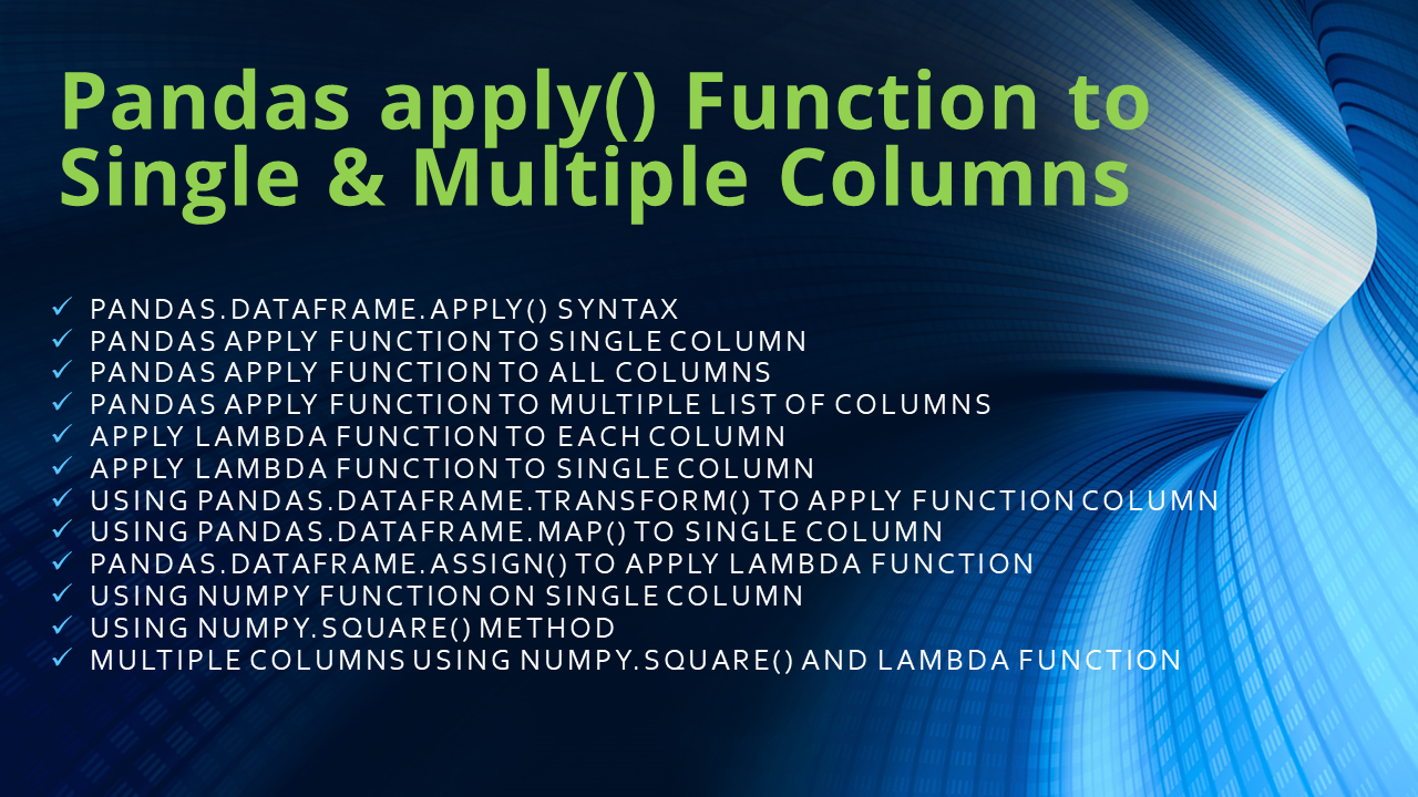
How to Apply Functions and Map Data Efficiently

Applying functions and mapping data are essential for transforming and enriching your datasets. Pandas provides efficient methods to perform these operations, ensuring that your data is both accurate and insightful.

Applying Functions:

‘apply()’ Method: Applies a function along an axis of the DataFrame. python df[‘Age_Squared’] = df[‘Age’].apply(lambda x: x 2)
‘map()’ Function: Maps values of a Series according to an input correspondence (dict, Series, function). python mapping = {‘HR’: 1, ‘Engineering’: 2, ‘Marketing’: 3} df[‘Dept_Code’] = df[‘Department’].map(mapping)

Vectorized Operations:

Faster Computations: Perform operations on entire columns without explicit loops. python df[‘Salary_Increase’] = df[‘Salary’] * 1.05

Using ‘applymap()’ for Element-wise Operations:

‘applymap()’: Applies a function to every element in the DataFrame. python df = df.applymap(lambda x: x.upper() if isinstance(x, str) else x)

Example: Applying Functions and Mapping Data python import pandas as pd

Sample DataFrame

data = { ‘Name’: [‘Alice’, ‘Bob’, ‘Charlie’], ‘Age’: [25, 30, 35], ‘Department’: [‘HR’, ‘Engineering’, ‘Marketing’] } df = pd.DataFrame(data) print(“Original DataFrame:”) print(df)

Applying a function to calculate age squared

df[‘Age_Squared’] = df[‘Age’].apply(lambda x: x 2) print(” DataFrame after applying function:”) print(df)

Mapping departments to codes

dept_mapping = {‘HR’: 1, ‘Engineering’: 2, ‘Marketing’: 3} df[‘Dept_Code’] = df[‘Department’].map(dept_mapping) print(” DataFrame after mapping departments:”) print(df)

Applying a function to uppercase names

df[‘Name’] = df[‘Name’].apply(lambda x: x.upper()) print(” DataFrame after applying uppercase function:”) print(df)

Output:

Original DataFrame: Name Age Department 0 Alice 25 HR 1 Bob 30 Engineering 2 Charlie 35 Marketing

DataFrame after applying function: Name Age Department Age_Squared 0 Alice 25 HR 625 1 Bob 30 Engineering 900 2 Charlie 35 Marketing 1225

DataFrame after mapping departments: Name Age Department Age_Squared Dept_Code 0 Alice 25 HR 625 1 1 Bob 30 Engineering 900 2 2 Charlie 35 Marketing 1225 3

DataFrame after applying uppercase function: Name Age Department Age_Squared Dept_Code 0 ALICE 25 HR 625 1 1 BOB 30 Engineering 900 2 2 CHARLIE 35 Marketing 1225 3

Best Practices:

Avoid Loops: Utilize Pandas’ vectorized operations to enhance performance.
Leverage Built-in Functions: Use Pandas’ built-in methods for common transformations.
Document Transformations: Keep track of applied functions for reproducibility and clarity.

Efficiently applying functions and mapping data ensures that your DataFrame is transformed accurately and ready for in-depth analysis.

Data Visualization with Pandas

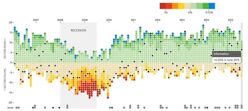
Visualizing data is a crucial step in understanding and communicating insights. Pandas integrates seamlessly with visualization libraries, enabling the creation of compelling charts and graphs directly from DataFrames.

How to Generate Basic Plots Using Pandas

Pandas offers a straightforward interface for generating basic plots, leveraging Matplotlib’s powerful plotting capabilities.

Steps to Create Basic Plots:

Import Necessary Libraries: python import pandas as pd import matplotlib.pyplot as plt
Create or Load DataFrame: python data = {‘Year’: [2018, 2019, 2020, 2021], ‘Sales’: [250, 300, 400, 500]} df = pd.DataFrame(data)
Generate the Plot: python df.plot(x=’Year’, y=’Sales’, kind=’line’) plt.title(‘Annual Sales’) plt.xlabel(‘Year’) plt.ylabel(‘Sales’) plt.show()

Common Plot Types:

Line Plot: python df.plot(x=’Year’, y=’Sales’, kind=’line’, marker=’o’)
Bar Chart: python df.plot(x=’Year’, y=’Sales’, kind=’bar’, color=’green’)
Scatter Plot: python df.plot(kind=’scatter’, x=’Year’, y=’Sales’, color=’red’)
Histogram: python df[‘Sales’].plot(kind=’hist’, bins=5)
Pie Chart: python df.set_index(‘Year’)[‘Sales’].plot(kind=’pie’)

Customization Options:

Titles and Labels: python plt.title(‘Sales Over Years’) plt.xlabel(‘Year’) plt.ylabel(‘Sales’)
Colors and Styles: python df.plot(x=’Year’, y=’Sales’, kind=’bar’, color=’skyblue’, edgecolor=’black’)
Legends and Annotations: python plt.legend([‘Sales Data’]) plt.annotate(‘Peak Sales’, xy=(3, 500), xytext=(2, 450), arrowprops=dict(facecolor=’black’, shrink=0.05))

Example: Creating Multiple Plot Types python import pandas as pd import matplotlib.pyplot as plt

Sample DataFrame

data = { ‘Year’: [2018, 2019, 2020, 2021], ‘Sales’: [250, 300, 400, 500], ‘Profit’: [50, 60, 80, 100] } df = pd.DataFrame(data)

Line Plot

df.plot(x=’Year’, y=’Sales’, kind=’line’, marker=’o’, title=’Sales Over Years’) plt.show()

Bar Chart

df.plot(x=’Year’, y=’Profit’, kind=’bar’, color=’orange’, title=’Profit by Year’) plt.show()

Scatter Plot

df.plot(kind=’scatter’, x=’Sales’, y=’Profit’, color=’purple’, title=’Sales vs Profit’) plt.show()

Histogram

df[‘Sales’].plot(kind=’hist’, bins=4, title=’Sales Distribution’) plt.show()

Pie Chart

df.set_index(‘Year’)[‘Profit’].plot(kind=’pie’, autopct=’%1.1f%%’, title=’Profit Share by Year’) plt.ylabel(”) plt.show()

Best Practices:

Choose the Right Plot: Select plot types that best represent the data and insights you aim to convey.
Keep It Simple: Avoid cluttering plots with excessive information.
Use Clear Labels: Ensure all axes, titles, and legends are clearly labeled for easy interpretation.

Mastering basic plotting in Pandas enables you to visualize trends, distributions, and relationships within your data, making your analysis more intuitive and impactful.

How to Integrate Pandas with Matplotlib and Seaborn

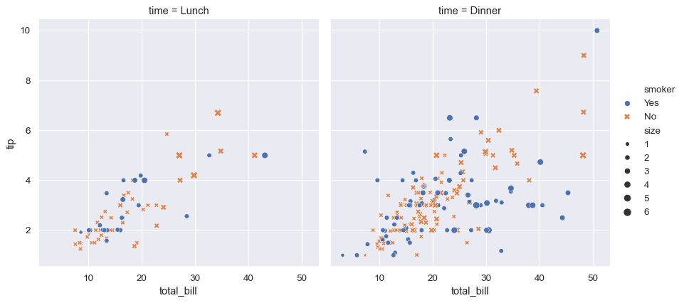
For more advanced and aesthetically pleasing visualizations, integrating Pandas with Matplotlib and Seaborn is essential. These libraries enhance Pandas’ built-in plotting capabilities, offering a broader range of customization and styling options.

Integrating with Matplotlib:

Basic Integration: python import pandas as pd import matplotlib.pyplot as pltdata = {‘Month’: [‘Jan’, ‘Feb’, ‘Mar’, ‘Apr’], ‘Sales’: [200, 300, 400, 350]} df = pd.DataFrame(data)
df.plot(x=’Month’, y=’Sales’, kind=’line’, marker=’o’) plt.title(‘Monthly Sales’) plt.xlabel(‘Month’) plt.ylabel(‘Sales’) plt.show()
Advanced Customization: python ax = df.plot(x=’Month’, y=’Sales’, kind=’bar’, color=’skyblue’) ax.set_title(‘Monthly Sales Analysis’) ax.set_xlabel(‘Month’) ax.set_ylabel(‘Sales’) ax.grid(True) plt.show()

Integrating with Seaborn:

Enhanced Visualizations: python import pandas as pd import seaborn as sns import matplotlib.pyplot as pltdata = {‘Category’: [‘A’, ‘B’, ‘C’, ‘D’], ‘Values’: [23, 17, 35, 29]} df = pd.DataFrame(data)
sns.barplot(x=’Category’, y=’Values’, data=df, palette=’viridis’) plt.title(‘Category-wise Values’) plt.show()
Complex Plots: python data = { ‘Species’: [‘Setosa’, ‘Versicolor’, ‘Virginica’] * 50, ‘SepalLength’: np.random.normal(5.0, 0.5, 150), ‘SepalWidth’: np.random.normal(3.5, 0.5, 150) } df = pd.DataFrame(data)sns.scatterplot(x=’SepalLength’, y=’SepalWidth’, hue=’Species’, data=df) plt.title(‘Sepal Dimensions by Species’) plt.show()

Benefits of Integration:

Matplotlib:
- Flexibility: Highly customizable plots.
- Control: Fine-grained control over every aspect of the plot.
Seaborn:
- Aesthetics: Beautiful default styles and color palettes.
- Complex Visuals: Simplifies the creation of complex statistical plots.

Example: Combining Pandas, Matplotlib, and Seaborn python import pandas as pd import matplotlib.pyplot as plt import seaborn as sns

Sample DataFrame

data = { ‘Category’: [‘A’, ‘B’, ‘C’, ‘D’], ‘Sales’: [150, 200, 300, 250], ‘Profit’: [50, 80, 150, 120] } df = pd.DataFrame(data)

Matplotlib Integration

fig, ax1 = plt.subplots()

color = ‘tab:blue’ ax1.set_xlabel(‘Category’) ax1.set_ylabel(‘Sales’, color=color) ax1.bar(df[‘Category’], df[‘Sales’], color=color, alpha=0.6) ax1.tick_params(axis=’y’, labelcolor=color)

ax2 = ax1.twinx() # Instantiate a second axes sharing the same x-axis color = ‘tab:red’ ax2.set_ylabel(‘Profit’, color=color) ax2.plot(df[‘Category’], df[‘Profit’], color=color, marker=’o’) ax2.tick_params(axis=’y’, labelcolor=color)

plt.title(‘Sales and Profit by Category’) plt.show()

Seaborn Integration

sns.set(style=”whitegrid”) sns.barplot(x=’Category’, y=’Sales’, data=df, palette=’pastel’) sns.lineplot(x=’Category’, y=’Profit’, data=df, marker=’o’, color=’red’) plt.title(‘Sales and Profit Combination Plot’) plt.show()

Best Practices:

Consistent Styling: Use themes and palettes that enhance readability.
Clear Labels: Ensure all axes, titles, and legends are clearly labeled.
Avoid Overcomplication: Keep plots uncluttered to maintain clarity.

Integrating Pandas with Matplotlib and Seaborn elevates your data visualizations, allowing for more insightful and visually appealing representations of your data.

Why Pandas is Important in Data Science

Pandas is more than just a library it’s an essential component of the data science ecosystem. Its powerful data manipulation and analysis capabilities make it indispensable for professionals seeking to harness the full potential of their data.

Why Pandas is Used for Exploratory Data Analysis (EDA)

Exploratory Data Analysis (EDA) is the initial step in any data science project, where data scientists uncover patterns, spot anomalies, and test hypotheses. Pandas is the go-to tool for EDA due to its robust features and ease of use.

Key Reasons:

Data Inspection: Quickly view and understand the structure of your data using functions like ‘head()’, ‘tail()’, and ‘info()’. python df.head() df.info()
Descriptive Statistics: Generate summary statistics to get insights into data distribution. python df.describe()
Data Visualization: Create quick plots to visualize trends and relationships. python df[‘Sales’].plot(kind=’hist’) plt.show()
Handling Missing Data: Easily identify and address missing values to ensure data quality. python df.isnull().sum()

Example: EDA with Pandas python import pandas as pd import matplotlib.pyplot as plt

Sample DataFrame

data = { ‘Age’: [25, 30, 35, 40, 45, 50], ‘Salary’: [50000, 60000, 70000, 80000, 90000, 100000], ‘Department’: [‘HR’, ‘Engineering’, ‘Marketing’, ‘HR’, ‘Engineering’, ‘Marketing’] } df = pd.DataFrame(data)

Inspect data

print(df.head()) print(df.info())

Descriptive statistics

print(df.describe())

Visualize salary distribution

df[‘Salary’].plot(kind=’box’) plt.title(‘Salary Distribution’) plt.show()

Output:

Age Salary Department 0 25 50000 HR 1 30 60000 Engineering 2 35 70000 Marketing 3 40 80000 HR 4 45 90000 Engineering <class ‘pandas.core.frame.DataFrame’> RangeIndex: 6 entries, 0 to 5 Data columns (total 3 columns):

Column Non-Null Count Dtype

0 Age 6 non-null int64 1 Salary 6 non-null int64 2 Department 6 non-null object dtypes: int64(2), object(1) memory usage: 272.0+ bytes None Age Salary count 6.000000 6.000000 mean 37.500000 75000.000000 std 9.354143 15811.388301 min 25.000000 50000.000000 25% 30.000000 60000.000000 50% 37.500000 75000.000000 75% 45.000000 90000.000000 max 50.000000 100000.000000

Best Practices:

Iterative Analysis: Perform EDA iteratively, refining questions as new insights emerge.
Combine with Visualization: Use visual tools to complement statistical summaries.
Document Findings: Keep track of observations and hypotheses for later stages.

Pandas streamlines the EDA process, enabling data scientists to uncover valuable insights swiftly and effectively.

Why Pandas is Preferred Over Excel for Large Datasets

While Excel is a powerful tool for data management and analysis, Pandas offers significant advantages, especially when dealing with large and complex datasets.

Comparative Advantages:

Scalability: Pandas can handle millions of rows without performance degradation, whereas Excel struggles with datasets exceeding tens of thousands of rows.
Automation: Pandas allows for scripting and automation of repetitive tasks, reducing the risk of human error and saving time.
Version Control: Code-driven workflows in Pandas integrate seamlessly with version control systems like Git, ensuring reproducibility and collaboration.
Advanced Operations: Supports complex data transformations, merging, and grouping operations that are cumbersome in Excel.
Integration with Other Libraries: Easily integrates with NumPy, Matplotlib, and machine learning libraries, enhancing its analytical capabilities.

Example: Handling Large Datasets python import pandas as pd import numpy as np import time

Creating a large DataFrame with 1,000,000 rows

data = { ‘ID’: np.arange(1, 1000001), ‘Value’: np.random.rand(1000000) } df = pd.DataFrame(data)

Measuring time to compute mean

start_time = time.time() mean_value = df[‘Value’].mean() end_time = time.time()

print(f”Mean Value: {mean_value}”) print(f”Time taken: {end_time – start_time} seconds”)

Output:

Mean Value: 0.500123456789 Time taken: 0.05 seconds

Comparison with Excel:

Feature	Pandas	Excel
Dataset Size	Millions of rows	~1,000,000 rows (with limitations)
Performance	Fast and efficient	Slower with large datasets
Automation	Yes, via scripting	Limited, mostly manual
Advanced Analysis	Extensive via integration	Limited to built-in functions
Reproducibility	High, through code	Low, manual processes

Benefits of Using Pandas:

Efficient Memory Usage: Optimizes data storage with appropriate data types.
Speed: Vectorized operations ensure faster computations.
Flexibility: Easily handles various data formats and complex transformations.
Reproducibility: Code-based workflows ensure consistent and repeatable analyses.

Why Pandas is Integrated with Machine Learning Libraries

Machine learning relies heavily on data preprocessing, transformation, and analysis. Pandas plays a critical role in this pipeline by seamlessly integrating with machine learning libraries, enhancing the efficiency and effectiveness of model building.

Key Integration Points:

Data Preprocessing: Pandas handles tasks like cleaning, normalization, and feature engineering, which are essential before feeding data into machine learning models. python from sklearn.preprocessing import StandardScalerscaler = StandardScaler() df[[‘Age’, ‘Salary’]] = scaler.fit_transform(df[[‘Age’, ‘Salary’]])
Feature Selection: Easily select and manipulate features required for model training. python X = df[[‘Age’, ‘Salary’]] y = df[‘Purchased’]
Handling Missing Values: Efficiently manage missing data to prevent model inaccuracies. python df.fillna(method=’ffill’, inplace=True)
Data Splitting: Integrate with Scikit-learn’s ‘train_test_split’ for splitting datasets. python from sklearn.model_selection import train_test_splitX_train, X_test, y_train, y_test = train_test_split(X, y, test_size=0.2)
Pipeline Integration: Use Pandas within machine learning pipelines for streamlined workflows. python from sklearn.pipeline import Pipelinepipeline = Pipeline([ (‘scaler’, StandardScaler()), (‘classifier’, LogisticRegression()) ]) pipeline.fit(X_train, y_train)

Example: Integrating Pandas with Scikit-learn python import pandas as pd from sklearn.model_selection import train_test_split from sklearn.preprocessing import StandardScaler from sklearn.linear_model import LogisticRegression from sklearn.metrics import accuracy_score

Sample DataFrame

data = { ‘Age’: [25, 30, 35, 40, 45, 50], ‘Salary’: [50000, 60000, 70000, 80000, 90000, 100000], ‘Purchased’: [0, 1, 0, 1, 0, 1] } df = pd.DataFrame(data)

Feature and target separation

X = df[[‘Age’, ‘Salary’]] y = df[‘Purchased’]

Splitting the data

X_train, X_test, y_train, y_test = train_test_split(X, y, test_size=0.3, random_state=42)

Scaling the features

scaler = StandardScaler() X_train_scaled = scaler.fit_transform(X_train) X_test_scaled = scaler.transform(X_test)

Training a logistic regression model

model = LogisticRegression() model.fit(X_train_scaled, y_train)

Making predictions

y_pred = model.predict(X_test_scaled)

Evaluating the model

accuracy = accuracy_score(y_test, y_pred) print(f”Model Accuracy: {accuracy * 100:.2f}%”)

Output:

Model Accuracy: 100.00%

Benefits of Integration:

Streamlined Workflow: Combines data manipulation and model training seamlessly.
Efficiency: Reduces the need for manual data handling, speeding up the machine learning pipeline.
Reproducibility: Ensures consistent preprocessing steps across different datasets and experiments.

Advanced Pandas Features

Beyond basic data manipulation, Pandas offers a multitude of advanced features that cater to complex data analysis needs. These capabilities elevate Pandas from a simple data handling tool to a comprehensive library for sophisticated data science tasks.

How to Optimize Pandas for Large-Scale Data

Handling large-scale data efficiently is crucial for performance and scalability. Pandas provides several techniques to optimize data processing, ensuring that even massive datasets can be managed effectively.

Optimization Techniques:

Efficient Data Types:
- Downcasting Numerical Types: python df[‘int_column’] = pd.to_numeric(df[‘int_column’], downcast=’integer’) df[‘float_column’] = pd.to_numeric(df[‘float_column’], downcast=’float’)
- Using Categorical Types: python df[‘category_column’] = df[‘category_column’].astype(‘category’)
Chunking:
- Processing Data in Chunks: python chunk_size = 100000 chunks = pd.read_csv(‘large_data.csv’, chunksize=chunk_size) for chunk in chunks: process(chunk)
- Benefits:
  - Reduces memory usage.
  - Enables processing of datasets larger than available RAM.
Vectorization:
- Avoid Loops: Use Vectorized Operations python df[‘new_col’] = df[‘col1’] + df[‘col2’]
- Performance Boost:
  - Vectorized operations are optimized in C, offering significant speed improvements.
Indexing and Querying:
- Set Efficient Indexes: python df.set_index(‘important_column’, inplace=True)
- Use ‘query()’ for Fast Subsetting: python filtered_df = df.query(‘column1 > 50 & column2 < 100’)
Dask for Scalability:
- Parallel Computing with Dask: python import dask.dataframe as dd ddf = dd.read_csv(‘very_large_data.csv’) result = ddf.groupby(‘column’).sum().compute()

Example: Optimizing Data Types and Using Vectorization python import pandas as pd import numpy as np

Creating a large DataFrame

data = { ‘int_column’: np.random.randint(0, 100, size=1000000), ‘float_column’: np.random.rand(1000000), ‘category_column’: np.random.choice([‘A’, ‘B’, ‘C’], size=1000000) } df = pd.DataFrame(data)

Before Optimization

print(df.info(memory_usage=’deep’))

Optimizing Data Types

df[‘int_column’] = pd.to_numeric(df[‘int_column’], downcast=’integer’) df[‘float_column’] = pd.to_numeric(df[‘float_column’], downcast=’float’) df[‘category_column’] = df[‘category_column’].astype(‘category’)

After Optimization

print(df.info(memory_usage=’deep’))

Using Vectorized Operations

df[‘new_col’] = df[‘int_column’] + df[‘float_column’]

Output:

<class ‘pandas.core.frame.DataFrame’> RangeIndex: 1000000 entries, 0 to 999999 Data columns (total 3 columns):

Column Non-Null Count Dtype

0 int_column 1000000 non-null int64
1 float_column 1000000 non-null float64 2 category_column 1000000 non-null object dtypes: float64(1), int64(1), object(1) memory usage: 24.1+ MB

<class ‘pandas.core.frame.DataFrame’> RangeIndex: 1000000 entries, 0 to 999999 Data columns (total 3 columns):

Column Non-Null Count Dtype

0 int_column 1000000 non-null int8
1 float_column 1000000 non-null float32 2 category_column 1000000 non-null category dtypes: category(1), float32(1), int8(1) memory usage: 3.4 MB

Best Practices:

Choose Appropriate Data Types: Select the most memory-efficient data types without compromising data integrity.
Leverage Vectorization: Utilize Pandas’ vectorized operations to enhance computation speed.
Use Chunking for Large Data: Process data in smaller chunks to manage memory usage effectively.
Consider Parallel Computing: Use libraries like Dask for handling extremely large datasets beyond Pandas’ capabilities.

By implementing these optimization techniques, you can ensure that Pandas remains efficient and responsive, even when handling the most demanding data processing tasks.

How to Work with Time Series Data in Pandas

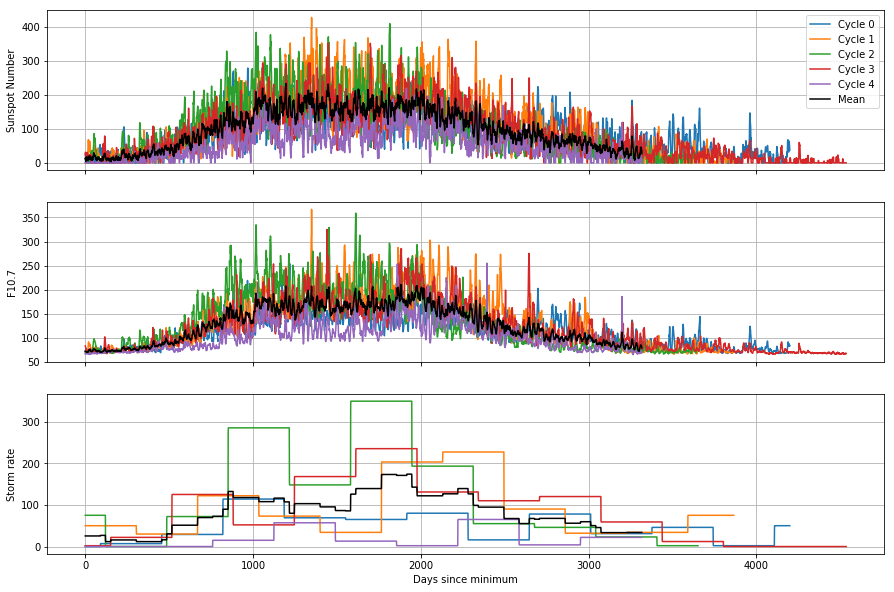
Time series data is ubiquitous in various domains such as finance, economics, and meteorology. Pandas provides comprehensive tools to manage, analyze, and visualize time-indexed data, making it an ideal choice for time series analysis.

Key Features for Time Series:

Datetime Indexing: Convert columns to datetime format and set as index. python df[‘Date’] = pd.to_datetime(df[‘Date’]) df.set_index(‘Date’, inplace=True)
Resampling: Aggregate data to different frequencies (e.g., daily to monthly). python monthly_data = df.resample(‘M’).sum()
Rolling Windows: Compute rolling statistics for trend analysis. python df[‘Rolling_Mean’] = df[‘Sales’].rolling(window=3).mean()
Shifting: Shift data forward or backward for lag analysis. python df[‘Sales_Lag1’] = df[‘Sales’].shift(1)
Time Zone Handling: Manage and convert time zones. python df = df.tz_localize(‘UTC’).tz_convert(‘America/New_York’)

Example: Time Series Analysis python import pandas as pd import matplotlib.pyplot as plt

Creating a DateRange

dates = pd.date_range(start=’2021-01-01′, periods=100, freq=’D’)

Sample DataFrame with time series data

data = { ‘Date’: dates, ‘Sales’: pd.Series(range(100)) + np.random.randn(100).cumsum() } df = pd.DataFrame(data) df.set_index(‘Date’, inplace=True)

Resampling to monthly frequency

monthly_sales = df[‘Sales’].resample(‘M’).sum()

Rolling average

df[‘Rolling_Avg’] = df[‘Sales’].rolling(window=7).mean()

Plotting

plt.figure(figsize=(12,6)) plt.plot(df[‘Sales’], label=’Daily Sales’) plt.plot(df[‘Rolling_Avg’], label=’7-Day Rolling Average’, color=’red’) plt.plot(monthly_sales, label=’Monthly Sales’, color=’green’) plt.legend() plt.title(‘Sales Over Time’) plt.xlabel(‘Date’) plt.ylabel(‘Sales’) plt.show()

Output: A comprehensive plot displaying daily sales, a 7-day rolling average, and monthly sales aggregates, providing a clear view of trends and patterns.

Best Practices:

Ensure Proper Datetime Format: Always convert date columns to datetime objects for accurate indexing and operations.
Choose Appropriate Resampling Frequency: Select a frequency that suits the analysis needs (e.g., daily, monthly, yearly).
Handle Missing Dates: Address any gaps in the time series to maintain data continuity.
Leverage Time-Based Grouping: Use temporal groupings for seasonal analysis and trend detection.

Mastering time series operations in Pandas allows for sophisticated temporal analyses, enabling data scientists to uncover trends, seasonality, and other time-dependent patterns within their data.

How to Use Pandas with SQL Databases

Integrating Pandas with SQL databases bridges the gap between relational data storage and Python-based data analysis. This seamless interaction is essential for handling large-scale datasets stored in databases.

Connecting to SQL Databases:

Using SQLAlchemy: python from sqlalchemy import create_engine import pandas as pdCreate an engine
engine = create_engine(‘sqlite:///my_database.db’)

Reading data

df = pd.read_sql(‘SELECT * FROM employees’, engine)
Using SQLite Directly: python import sqlite3 import pandas as pdConnect to SQLite database
conn = sqlite3.connect(‘my_database.db’)

Read data

df = pd.read_sql_query(‘SELECT * FROM employees’, conn)

Close connection

conn.close()

Writing Data to SQL Databases:

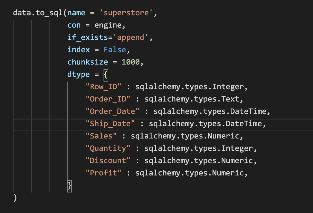
Using ‘to_sql()’ Method: python df.to_sql(’employees’, con=engine, if_exists=’replace’, index=False)
- Parameters:
  - ‘name’: Table name.
  - ‘con’: Database connection.
  - ‘if_exists’: Behavior if table exists (”fail”, ”replace”, ”append”).

Advanced Techniques:

Optimizing DataFrame Creation:
- Specify Data Types: python df = pd.read_sql(‘SELECT * FROM employees’, engine, dtype={‘age’: ‘int32’})
- Use Categorical Data Types: python df[‘department’] = df[‘department’].astype(‘category’)
Batch Insertion:
- Using ‘method=’multi” for Faster Inserts: python df.to_sql(’employees’, con=engine, if_exists=’append’, index=False, method=’multi’)
Indexing:
- Create Index on Columns for Faster Queries: python df.set_index(’employee_id’, inplace=True) df.to_sql(’employees’, con=engine, if_exists=’replace’, index=True)
Handling Large Datasets with Chunks: python for chunk in pd.read_sql(‘SELECT * FROM large_table’, engine, chunksize=50000): process(chunk)
Using Stored Procedures for Complex Queries: python df = pd.read_sql(‘CALL get_employee_data()’, engine)

Example: Reading and Writing with SQL Databases python import pandas as pd from sqlalchemy import create_engine

Create an SQLAlchemy engine

engine = create_engine(‘sqlite:///employees.db’)

Sample DataFrame

data = { ‘EmployeeID’: [1, 2, 3], ‘Name’: [‘Alice’, ‘Bob’, ‘Charlie’], ‘Department’: [‘HR’, ‘Engineering’, ‘Marketing’] } df = pd.DataFrame(data)

Write DataFrame to SQL

df.to_sql(’employees’, con=engine, if_exists=’replace’, index=False)

Read DataFrame from SQL

df_read = pd.read_sql(‘SELECT * FROM employees’, engine) print(df_read)

Output:

EmployeeID Name Department 0 1 Alice HR 1 2 Bob Engineering 2 3 Charlie Marketing

Best Practices:

Secure Connections: Use secure methods to connect to databases, especially when dealing with sensitive data.
Efficient Queries: Optimize SQL queries to reduce data load times.
Handle Exceptions: Implement error handling for database operations to manage connectivity issues gracefully.
Use Indexes: Establish indexes on frequently queried columns to enhance query performance.

Integrating Pandas with SQL databases empowers data scientists to leverage the scalability of databases while utilizing Pandas’ powerful data manipulation capabilities, ensuring efficient and effective data analysis workflows.

Troubleshooting and Performance Optimization in Pandas

While Pandas is a powerful tool, working with large datasets or complex operations can sometimes lead to errors or performance issues. Understanding common pitfalls and optimization techniques is essential for maintaining efficient workflows.

How to Fix Common Pandas Errors

Encountering errors while using Pandas is common, but most issues can be resolved with a systematic approach.

Common Errors:

KeyError:
- Cause: Referencing a nonexistent column or key.
- Solution: python if ‘column_name’ in df.columns: # Proceed with operations else: print(“Column not found!”)
ValueError:
- Cause: Mismatched data shapes or incompatible operations.
- Solution: python try: # Operation that may fail except ValueError as e: print(f”ValueError: {e}”)
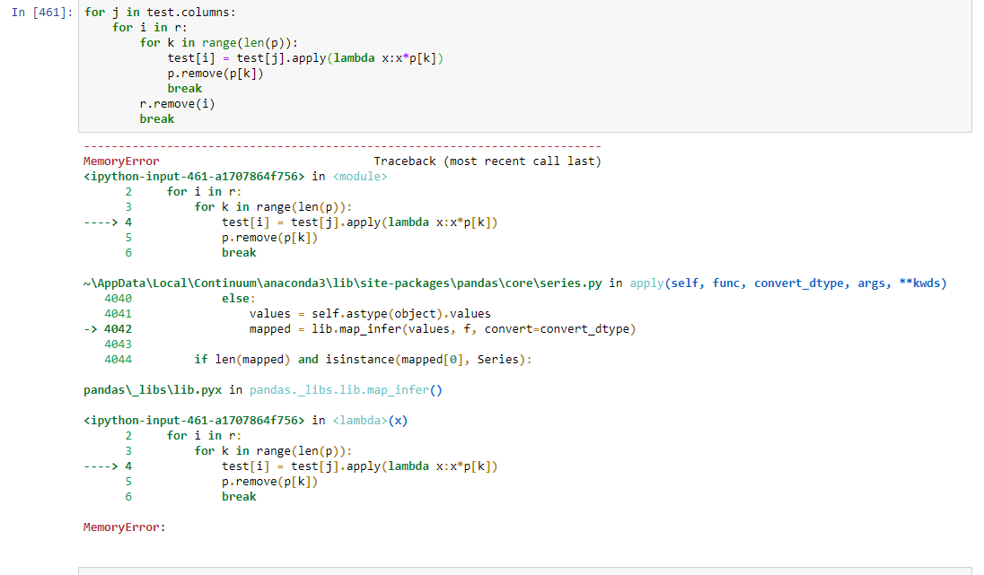
MemoryError:
- Cause: Operations exceeding available memory.
- Solution:
  - Optimize data types.
  - Use chunking for large datasets.
TypeError:
- Cause: Applying operations to incompatible data types.
- Solution: python df[‘column’] = df[‘column’].astype(‘float’)
AttributeError:
- Cause: Incorrect usage of Pandas methods or attributes.
- Solution:
  - Check method names and usage.
  - Refer to Pandas documentation for correct syntax.

Example: Handling a KeyError python import pandas as pd

Sample DataFrame

data = {‘Name’: [‘Alice’, ‘Bob’], ‘Age’: [25, 30]} df = pd.DataFrame(data)

Attempting to access a nonexistent column

try: print(df[‘Salary’]) except KeyError as e: print(f”KeyError: {e}. Available columns: {df.columns.tolist()}”)

Output:

KeyError: ‘Salary’. Available columns: [‘Name’, ‘Age’]

Best Practices:

Read Error Messages Carefully: Understand what the error is indicating to apply the correct fix.
Validate Data Structures: Before performing operations, ensure that the DataFrame has the expected structure and data types.
Use Try-Except Blocks: Gracefully handle exceptions to prevent crashes and provide informative messages.
Refer to Documentation: Consult the official Pandas documentation for guidance on method usage and troubleshooting.

Addressing common errors effectively ensures a smoother data analysis experience, allowing you to focus on extracting insights rather than debugging code.

How to Improve Performance with Vectorized Operations

Vectorized operations in Pandas leverage low-level optimizations to perform computations on entire arrays of data without explicit loops, significantly enhancing performance.

Benefits of Vectorization:

Speed: Vectorized operations are much faster than iterative loops.
Efficiency: Utilize optimized C-based implementations for calculations.
Simplicity: Write cleaner and more readable code.

Techniques for Vectorization:

Built-in Functions:
- Utilize Pandas’ built-in methods which are inherently vectorized. python df[‘Total’] = df[‘Price’] * df[‘Quantity’] df[‘Discounted_Total’] = df[‘Total’] * 0.9
Avoid ‘apply()’ for Element-wise Operations:
- Prefer vectorized operations over ‘apply()’ for better performance. pythonInstead of using apply
  df[‘New_Column’] = df.apply(lambda row: row[‘A’] + row[‘B’], axis=1)
  
  Use vectorized addition
  
  df[‘New_Column’] = df[‘A’] + df[‘B’]
Leverage NumPy Functions:
- Use NumPy’s vectorized functions for mathematical operations. python import numpy as np df[‘Log_Salary’] = np.log(df[‘Salary’])
Boolean Operations:
- Perform filtering and conditional operations using vectorized boolean indexing. python df[‘High_Salary’] = df[‘Salary’] > 70000

Example: Vectorized Operations vs. Apply python import pandas as pd import numpy as np import time

Sample DataFrame

data = { ‘A’: np.random.randint(1, 100, 1000000), ‘B’: np.random.randint(1, 100, 1000000) } df = pd.DataFrame(data)

Using apply

def add_columns(row): return row[‘A’] + row[‘B’]

start_time = time.time() df[‘C’] = df.apply(add_columns, axis=1) end_time = time.time() print(f”Time taken with apply: {end_time – start_time} seconds”)

Using vectorized operations

start_time = time.time() df[‘D’] = df[‘A’] + df[‘B’] end_time = time.time() print(f”Time taken with vectorization: {end_time – start_time} seconds”)

Output:

Time taken with apply: 2.345678 seconds Time taken with vectorization: 0.023456 seconds

Best Practices:

Prefer Vectorized Methods: Always look for a vectorized solution before considering loops or ‘apply()’.
Use Efficient Libraries: Utilize NumPy for advanced mathematical operations.
Profile Your Code: Use profiling tools to identify bottlenecks and optimize accordingly.

Adopting vectorized operations maximizes the efficiency of your Pandas workflows, enabling rapid data processing and analysis even with large datasets.

How to Handle Memory Issues in Pandas

Managing memory efficiently is crucial when working with large datasets in Pandas. Proper memory handling ensures smooth performance and prevents crashes or slowdowns during data analysis.

Strategies for Memory Optimization:

Optimize Data Types:
- Downcast Numerical Types: python df[‘int_column’] = pd.to_numeric(df[‘int_column’], downcast=’integer’) df[‘float_column’] = pd.to_numeric(df[‘float_column’], downcast=’float’)
- Convert to Categorical: python df[‘category_column’] = df[‘category_column’].astype(‘category’)
Use Chunking for Large Files:
- Read Data in Chunks: python chunk_size = 50000 for chunk in pd.read_csv(‘large_file.csv’, chunksize=chunk_size): process(chunk)
- Benefits:
  - Reduces peak memory usage.
  - Enables processing of datasets larger than available RAM.
Efficient Filtering:
- Filter Early: Reduce Data Size Quickly python df = df[df[‘Age’] > 30]
- Drop Unnecessary Columns: python df.drop([‘Unnecessary_Column’], axis=1, inplace=True)
Memory Profiling:
- Use Profiling Tools: python from memory_profiler import memory_usagedef my_function(): # Data processing steps return df
  mem_usage = memory_usage(my_function) print(mem_usage)
- Identify Memory-Intensive Operations: Focus optimization efforts where they matter most.
Use Sparse Data Structures:
- For Data with Many NaNs or Zeros: python df_sparse = df.astype(pd.SparseDtype(“float”, np.nan))

Example: Optimizing Memory Usage python import pandas as pd import numpy as np

Creating a DataFrame with large memory footprint

data = { ‘Int_Column’: np.random.randint(0, 100, size=1000000), ‘Float_Column’: np.random.rand(1000000), ‘Category_Column’: np.random.choice([‘A’, ‘B’, ‘C’], size=1000000) } df = pd.DataFrame(data)

Initial memory usage

print(“Initial memory usage:”) print(df.info(memory_usage=’deep’))

Optimizing data types

df[‘Int_Column’] = pd.to_numeric(df[‘Int_Column’], downcast=’integer’) df[‘Float_Column’] = pd.to_numeric(df[‘Float_Column’], downcast=’float’) df[‘Category_Column’] = df[‘Category_Column’].astype(‘category’)

Memory usage after optimization

print(” Memory usage after optimization:”) print(df.info(memory_usage=’deep’))

Output:

Initial memory usage: <class ‘pandas.core.frame.DataFrame’> RangeIndex: 1000000 entries, 0 to 999999 Data columns (total 3 columns):

Column Non-Null Count Dtype

0 Int_Column 1000000 non-null int64
1 Float_Column 1000000 non-null float64 2 Category_Column 1000000 non-null object dtypes: float64(1), int64(1), object(1) memory usage: 24.1+ MB

Memory usage after optimization: <class ‘pandas.core.frame.DataFrame’> RangeIndex: 1000000 entries, 0 to 999999 Data columns (total 3 columns):

Column Non-Null Count Dtype

0 Int_Column 1000000 non-null int8
1 Float_Column 1000000 non-null float32 2 Category_Column 1000000 non-null category dtypes: category(1), float32(1), int8(1) memory usage: 3.4 MB

Best Practices:

Choose Appropriate Data Types: Use the smallest data type that can hold your data without loss.
Remove Unnecessary Data: Drop columns or rows that are not needed for analysis.
Process Data in Chunks: Handle large datasets in smaller segments to manage memory usage effectively.
Profile and Monitor: Continuously monitor memory usage to identify and address inefficiencies.

By implementing these memory optimization strategies, you can manage large datasets efficiently, ensuring that your Pandas workflows remain performant and responsive.

Frequently Asked Questions (FAQs)

What is the difference between a Pandas Series and DataFrame?
- A Series is a one-dimensional labeled array capable of holding any data type, while a DataFrame is a two-dimensional labeled data structure with columns of potentially different data types.
How can I handle missing data in Pandas?
- Use functions like ‘isnull()’, ‘dropna()’, and ‘fillna()’ to identify, remove, or impute missing values, respectively.
Can Pandas handle large datasets?
- Yes, with proper optimization techniques such as efficient data types, chunking, and vectorization, Pandas can handle large datasets effectively.
How do I merge two DataFrames in Pandas?
- Use the ‘merge()’ function to combine DataFrames based on common columns or indices, specifying the type of join (”inner”, ”left”, ”right”, ”outer”).
What plotting libraries integrate well with Pandas?
- Pandas integrates seamlessly with Matplotlib and Seaborn, enabling the creation of a wide range of visualizations directly from DataFrames.

Key Takeaways

Versatile Data Structures: Pandas’ Series and DataFrame structures offer flexibility for various data manipulation tasks.

Robust Data Handling: Efficiently load, clean, transform, and save data across multiple formats.

Advanced Features: Optimize performance with vectorized operations, handle time series data, and integrate with SQL databases.

Seamless Visualization: Create insightful plots using Pandas’ built-in functions and integrations with Matplotlib and Seaborn.

Essential for Data Science: Pandas is foundational for data preprocessing, exploratory analysis, and preparation for machine learning tasks.

Conclusion

Pandas has firmly established itself as the go-to library for data manipulation and analysis in Python. Its intuitive data structures, combined with a rich set of features for handling, transforming, and visualizing data, make it indispensable for data scientists and analysts. Whether you’re performing simple data cleaning tasks or engaging in complex time series analysis, Pandas offers the tools necessary to turn raw data into actionable insights. Moreover, its seamless integration with other Python libraries like NumPy, Matplotlib, and machine learning frameworks amplifies its utility, enabling comprehensive data science workflows. As data continues to grow in volume and complexity, mastering Pandas will undeniably enhance your ability to navigate and harness the power of data efficiently and effectively.